The Hangar
Complete, runnable aircraft — climb in and turn the key. The first squadron ships inside the package as modules; the rest are copy-paste recipes. SI units everywhere, as always.
The shipped squadron
| Script | Run | What it flies |
|---|---|---|
| Feature tour | python -m ikarus.examples.feature_tour |
The full airshow: TiO₂ cross metasurface — materials, structure plots, order-resolved efficiencies, field maps, spectrum, circular polarization, HDF5. Output lands in ikarus_tour_output/. |
| Grating diffraction | python -m ikarus.examples.grating_diffraction |
1-D TiO₂ binary grating; propagating orders + exit angles vs. wavelength. |
| Metasurface spectrum | python -m ikarus.examples.metasurface_spectrum |
R/T spectrum of a 2-D meta-atom. |
| Inverse metamirror | python -m ikarus.examples.inverse_metamirror |
A GA evolves a reflective meta-atom. |
| Fresnel validation | python -m ikarus.examples.validation_fresnel |
The machine-precision sanity anchor. |
| Save & load | python -m ikarus.examples.save_load |
Write a result to HDF5 (totals, orders, metadata, fields) and load it back. |
Fresnel validation — the trust anchor
Before believing any solver, make it reproduce something you can derive by hand. One interface, analytic answer, fifteen decimal places:
import numpy as np
from ikarus import RCWA

rcwa = RCWA(period_x=1e-6, period_y=1e-6, n_orders=0)   # specular only
rcwa.add_uniform_layer(np.inf, 1.0)      # air
rcwa.add_uniform_layer(np.inf, 1.5)      # glass (constant index)

rcwa.set_source(wavelength=600e-9, theta=0, polarization="linear")
_, _, res = rcwa.simulate()

R_fresnel = ((1.0 - 1.5) / (1.0 + 1.5)) ** 2
print(f"Ikarus  R = {res.R_total:.12f}")
print(f"Fresnel R = {R_fresnel:.12f}")
print(f"|diff| = {abs(res.R_total - R_fresnel):.2e}")   # ~1e-15
Anti-reflection thin film — the classic
The quarter-wave trick, in eight lines:
import numpy as np
from ikarus import RCWA

n_film, lam0 = 1.23, 550e-9          # ideal AR index ≈ sqrt(1.5)
d = lam0 / (4 * n_film)              # quarter-wave thickness

rcwa = RCWA(period_x=1e-6, period_y=1e-6, n_orders=0)
rcwa.add_uniform_layer(np.inf, 1.0)
rcwa.add_uniform_layer(d, n_film)
rcwa.add_uniform_layer(np.inf, 1.5)

for wl in (450e-9, 550e-9, 650e-9):
    rcwa.set_source(wavelength=wl, theta=0, polarization="linear")
    print(f"{wl*1e9:.0f} nm: R = {rcwa.simulate()[2].R_total:.4f}")
# the minimum sits at 550 nm, as designed
Guided-mode resonance filter — the drama queen
A high-index grating that doubles as a waveguide: at just the right wavelength the light couples in, circulates, and exits as a needle-sharp reflection peak.
import numpy as np
from ikarus import RCWA

period = 880e-9
rcwa = RCWA(period_x=period, period_y=period, resolution=(256, 2), n_orders=(25, 0))

topo = np.zeros((200, 2), dtype=int)
topo[:100, :] = 1                     # 50% duty cycle
rcwa.add_uniform_layer(np.inf, "Air")
rcwa.add_layer(180e-9, topo, ["Si3N4", "Air"])
rcwa.add_uniform_layer(np.inf, "SiO2")

for wl in np.linspace(1.0e-6, 1.1e-6, 11):
    rcwa.set_source(wavelength=wl, theta=0, polarization="linear", linear_pol_angle=0)
    print(f"{wl*1e9:.0f} nm: R = {rcwa.simulate()[2].R_total:.3f}")
    # a narrow resonance spikes inside the band
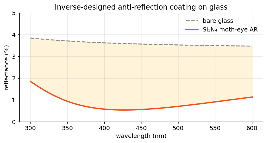
Inverse design: AR coating
No solid material has the n ≈ 1.21 a glass AR coating wants — so let evolution build one out of structure: a subwavelength Si₃N₄ moth-eye whose fill fraction fakes the unattainable index. Broadband 300–600 nm, worst-case optimized:
import os
for v in ("OMP_NUM_THREADS", "OPENBLAS_NUM_THREADS", "MKL_NUM_THREADS"):
    os.environ.setdefault(v, "1")        # single-thread BLAS for the tight loop

import numpy as np
from ikarus.inverse import MetaAtom, free, pixels, Target, optimize

atom = MetaAtom(period=180e-9, cover="Air", substrate="SiO2")
atom.add_pattern(topology=pixels(8, 8, symmetry="c4v"),
                 materials=["Air", "Si3N4"], height=free(40e-9, 200e-9))

target = Target.minimize("R", band=(300e-9, 600e-9, 6), worst_case=True)
best = optimize(atom, target, n_orders=6, pop=16, n_gen=10, seed=0)
print(best.report())

coating = best.metaatom
wl = np.linspace(300e-9, 600e-9, 13)
R = []
for w in wl:
    coating.set_source(wavelength=w, theta=0, polarization="linear")
    R.append(coating.simulate()[2].R_total)
print("worst-case R:", f"{max(R)*100:.2f}%")     # ~1.5% vs ~3.8% bare glass

# plot the AR coating vs. bare glass
import matplotlib.pyplot as plt
from ikarus import default_library
n_sub = np.array([complex(default_library.get("SiO2", w)).real for w in wl])
R_bare = ((n_sub - 1) / (n_sub + 1)) ** 2
plt.figure(figsize=(7, 4))
plt.plot(wl * 1e9, R_bare * 100, "--", color="0.6", label="bare glass")
plt.plot(wl * 1e9, np.array(R) * 100, lw=2, color="C1", label="moth-eye AR")
plt.xlabel("wavelength (nm)"); plt.ylabel("reflectance (%)"); plt.ylim(bottom=0)
plt.legend(); plt.grid(alpha=0.3)
plt.tight_layout(); plt.savefig("ar_coating.png", dpi=150, bbox_inches="tight")
plt.show()
Beam deflector — power steering
Maximize power into the +1 reflected order at 1550 nm:
import os
os.environ.setdefault("OMP_NUM_THREADS", "1")
from ikarus.inverse import MetaAtom, free, pixels, Target, optimize

atom = MetaAtom(period=1.2e-6, cover="Air", substrate="SiO2")
atom.add_pattern(topology=pixels(48, 8, symmetry="mirror_y"),
                 materials=["Air", "Si"], height=free(0.2e-6, 0.6e-6))

# pixels + a free height are differentiable, so optimize() automatically uses
# adjoint gradients here -- 200 pixel DOFs cost the same as 4.
best = optimize(atom, Target.maximize("R", order=(1, 0), at=1550e-9),
                n_orders=(12, 4), min_feature=100e-9)
print(best.report())
Save & load results
A simulation is expensive; its result shouldn't evaporate when the script ends.
Ikarus writes results to a self-describing HDF5 file — totals, per-order
efficiencies, exit angles, the full geometry/source metadata, and (optionally)
reconstructed fields — that any HDF5 tool (h5py, h5ls, HDFView) can read, and
that loads back into a plain dict with no RCWA object required.
Needs the io extra
pip install "ikarus-rcwa[io]" (h5py).
Save the most recent (or a supplied) result. include picks what goes in —
add "fields" to store a reconstructed cross-section too:
import numpy as np
from ikarus import RCWA, shapes

period, N = 500e-9, 96
rcwa = RCWA(period_x=period, period_y=period, resolution=(N, N), n_orders=(8, 8))
rcwa.add_uniform_layer(np.inf, "Air")
rcwa.add_layer(220e-9, shapes.circle(radius=0.3, grid_shape=(N, N)), ["Air", "TiO2"])
rcwa.add_uniform_layer(np.inf, "SiO2")
rcwa.set_source(wavelength=600e-9, theta=10, polarization="linear")
_, _, result = rcwa.simulate()

rcwa.save_results("metasurface.h5",
                  include=["T", "R", "metadata", "fields"], result=result)
Load it back later — anywhere, no solver state needed:
from ikarus import RCWA

data = RCWA.load_results("metasurface.h5")        # a nested dict

print(f"R = {data['R_total']:.4f}   T = {data['T_total']:.4f}")
meta = data["metadata"]
print("period:", meta["period_x"], "  source:", meta["source"]["wavelength"])

# per-order data round-trips too:
p, q, t = data["order_p"], data["order_q"], data["T_orders"]
for i in np.argsort(-t)[:3]:
    print(f"order ({p[i]:+d},{q[i]:+d}): T = {t[i]:.4f}")
Running the shipped python -m ikarus.examples.save_load prints:
computed:  R = 0.1114   T = 0.8886
saved   -> ikarus_save_load_output/metasurface.h5  (418 KB)

file contents: R, R_orders, R_total, T, T_orders, T_total, energy_balance,
fields/xz/E, fields/xz/H, fields/xz/coord_x, fields/xz/coord_z, metadata,
order_p, order_q, phi_out_ref, phi_out_trn, theta_out_ref, theta_out_trn

loaded:    R_total = 0.1114   T_total = 0.8886
geometry:  period = 500 nm, n_orders = (8, 8)
source:    lambda = 600 nm, theta = 10 deg, pol = linear
brightest transmitted orders:
   (+0,+0): T = 0.2751
   (-1,+0): T = 0.1946
   (+1,+0): T = 0.1726

round-trip verified: loaded values match the originals exactly.
What's in the file
| Group / dataset | Contents |
|---|---|
R_total, T_total, energy_balance |
scalar totals |
R, T |
complex zero-order coefficients (or a co/cross group for circular polarization) |
R_orders, T_orders |
per-order efficiencies |
order_p, order_q |
the (p, q) order labels |
theta_out_*, phi_out_* |
per-order exit angles (deg) |
metadata |
JSON: periods, n_orders, resolution, the layer stack, and the source |
fields/... |
reconstructed E/H + coordinates (only if "fields" was included) |
Sweeps and archives
To archive a whole Sweep, save each point in a loop
(save_results(f"run_{i}.h5", result=res)), or stack the arrays you care
about (res.R_total, res.axes) with numpy.savez. For a single design,
one HDF5 file with include=["T","R","metadata","fields"] captures everything
needed to reproduce and re-plot it later. Full API:
Tools → HDF5 I/O.
Continue exploring: Flight School for the step-by-step versions · API Reference for every knob · Need for Speed for making big runs fast.