Lesson 6 · Coming in at an Angle

Mission: tilt the illumination, paint an angle–wavelength dispersion map, and learn to recognize a Rayleigh–Wood anomaly when one streaks across your plot.

Tilting the source

theta tilts from straight-down (+z), phi picks the compass direction of the tilt. The sweep pattern is the same golden one — touch only the source:

import numpy as np
from ikarus import RCWA, shapes

period, N = 500e-9, 96
disk = shapes.circle(radius=0.3, grid_shape=(N, N))
rcwa = RCWA(period_x=period, period_y=period, resolution=(N, N), n_orders=(10, 10))
rcwa.add_uniform_layer(np.inf, "Air")
rcwa.add_layer(180e-9, disk, ["Air", "TiO2"])
rcwa.add_uniform_layer(np.inf, "SiO2")

thetas = np.linspace(0, 60, 61)
R = np.empty_like(thetas)
for i, th in enumerate(thetas):
    rcwa.set_source(wavelength=600e-9, theta=th, phi=0,
                    polarization="linear", linear_pol_angle=90)
    R[i] = rcwa.simulate()[2].R_total      # TM: watch for the Brewster dip

Conical incidence comes free

A non-zero phi swings the plane of incidence out of x–z (conical mounting). No special flags — once theta > 0, the full 2-D harmonic machinery is engaged anyway.

The dispersion map

The single most informative plot for any periodic structure: reflectance over (wavelength, angle). Resonances trace dispersive bands; diffraction onsets cut sharp lines:

import numpy as np
from ikarus import RCWA, shapes

period, N = 500e-9, 96
disk = shapes.circle(radius=0.3, grid_shape=(N, N))
rcwa = RCWA(period_x=period, period_y=period, resolution=(N, N), n_orders=(10, 10))
rcwa.add_uniform_layer(np.inf, "Air")
rcwa.add_layer(180e-9, disk, ["Air", "TiO2"])
rcwa.add_uniform_layer(np.inf, "SiO2")

wavelengths = np.linspace(450e-9, 750e-9, 80)
thetas = np.linspace(0, 50, 60)
Rmap = np.empty((thetas.size, wavelengths.size))
for j, th in enumerate(thetas):
    for i, wl in enumerate(wavelengths):
        rcwa.set_source(wavelength=wl, theta=th, polarization="linear")
        Rmap[j, i] = rcwa.simulate()[2].R_total

import matplotlib.pyplot as plt
plt.pcolormesh(wavelengths * 1e9, thetas, Rmap, shading="auto", cmap="magma")
plt.xlabel("wavelength (nm)"); plt.ylabel("incidence angle (deg)")
plt.colorbar(label="Reflectance"); plt.savefig("dispersion.png", dpi=150)

Angle–wavelength reflectance map of a TiO₂ metasurface; the bright streaks are Rayleigh–Wood anomalies, where diffraction orders cut on.

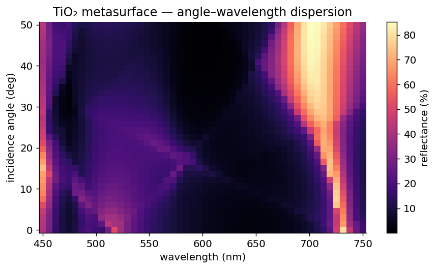
Spotting Rayleigh–Wood anomalies

A diffraction lane opens (or closes) when its in-plane wavevector touches the light line. For the first order into the cover (index \(n_c\)) at \(\phi = 0\):

\[ n_c\,\sin\theta + \frac{\lambda}{\Lambda} = n_c \quad\Rightarrow\quad \lambda_{\text{RW}} = \Lambda\,n_c\,(1 - \sin\theta). \]

Those are the bright cusps streaking across your map — a new lane opening and briefly rearranging all the traffic. Ikarus regularizes orders sitting exactly on the light line with a vanishing imaginary loss, so the solve stays well-posed straight through the anomaly; just expect the local energy defect to tick up and convergence to slow there.

# Watch the lane count grow with angle:
for th in (0, 20, 40):
    rcwa.set_source(wavelength=600e-9, theta=th, polarization="linear")
    _, _, res = rcwa.simulate()
    n_prop = int(np.sum(np.isfinite(res.theta_out_ref) & (res.R_orders > 1e-6)))
    print(f"theta={th:2d} deg: {n_prop} propagating reflected orders")

Expected results

• Smooth specular response at small angles; a Brewster-like TM dip.
• Wood anomalies as bright curves \(\lambda_{\text{RW}}(\theta)\) across the dispersion map, with the order count changing as you cross them.

Pilot habits

• Re-run the convergence ritual at your largest angle — oblique incidence populates more orders.
• Mask NaN exit angles (np.isfinite) before plotting angle data.
• Near an anomaly, a slightly larger energy defect is expected; refine n_orders only if your metric lives there.

---

Next — the finale: Lesson 7 · Designing the Shape Itself →