How RCWA Works
Or: the biography of a photon entering a periodic obstacle course.
This chapter explains rigorous coupled-wave analysis (RCWA, also known as the Fourier Modal Method) the way we wish someone had explained it to us: intuition first, machinery second, full mathematics on demand. Nothing here is hand-wavy in the end — every analogy is backed by the exact equations Ikarus implements, and the conventions are stated precisely so you can audit the code.
RCWA in one breath
Take a structure that repeats in \(x\) and \(y\) and is built from flat slabs in \(z\). Describe the light in each slab as a sum of a few hundred plane waves (Fourier harmonics). Inside each slab, find the field patterns that travel without changing shape (eigenmodes). Then do impeccable bookkeeping on how those modes bounce and transmit at every interface (scattering matrices). That's it. That's the whole method.
No mesh. No time stepping. The field is handled analytically in \(z\) and spectrally in \((x, y)\) — which is why RCWA wins so decisively for gratings, metasurfaces and photonic-crystal slabs: those structures are literally stacks of patterned slabs, and the answers you usually want (efficiency per diffraction order, phase, exit angles) fall out natively.

Part I — The story (no math yet)
A plane wave meets a periodic world
Picture a perfectly flat wave of light gliding down toward a surface that repeats every few hundred nanometers — a grating, say. The wave can't ignore the pattern, but it also can't respond arbitrarily: periodicity is a contract. Whatever the field does, it must repeat (up to a phase twist) with the same period as the structure. That's Bloch's theorem, and it has a beautiful consequence:
The light can only leave in a discrete set of directions.
Think of them as exit lanes. Lane \((0,0)\) is the specular direction — straight reflection/transmission, the only lane a flat mirror offers. The pattern opens additional lanes at angles set purely by geometry: the wavelength-to-period ratio. Each lane is a diffraction order, labelled by integers \((m, n)\), and RCWA's headline output is simply how much power went down each lane, and with what phase.
Some lanes are special: if the geometry asks a lane to leave at "more than 90°", that order can't propagate — it becomes evanescent, a ghost wave that clings to the surface and decays exponentially. Ghost lanes carry no power to the far field, but they matter enormously inside the structure: near-field coupling between layers travels through them.
Every periodic pattern is a sum of smooth waves
How do we describe the patterned material itself? The same way audio engineers
describe a sound: as a sum of pure tones. A square pillar, a ring, a
freeform inverse-designed blob — every periodic permittivity profile
\(\varepsilon(x, y)\) is a sum of perfectly smooth spatial waves (Fourier
components). Keep the first \(M\) harmonics in each direction and you have a
controllable approximation: more harmonics, sharper edges, higher cost. The
single number n_orders you pass to Ikarus is exactly this truncation.
Each slab has natural gaits
Inside one uniform-in-\(z\) slab, Maxwell's equations admit special field patterns that propagate without changing shape — only their amplitude and phase evolve, exponentially, with depth. These are the slab's eigenmodes: its natural gaits. Any field in the slab is a mixture of gaits walking down plus gaits walking up. Finding them costs one dense eigendecomposition per patterned layer — the computational heart of RCWA.
The bookkeeping that doesn't melt
Now stack the slabs. At every interface, gaits of one slab convert into gaits of the next — partially transmitted, partially reflected, with infinite internal ping-pong between interfaces. Two ways to track this:
- Transfer matrices push the field through the stack, multiplying layer by layer. Elegant — and doomed. They carry growing exponentials \(e^{+\lambda z}\) for evanescent modes, which overflow double precision the moment a layer is thick or a mode decays fast. This is the numerical wax melting in mid-flight.
- Scattering matrices ask each layer a humbler question: "if light knocks on your door from either side, what comes back and what goes through?" Every entry involves only decaying exponentials \(e^{-\lambda L}\) — bounded by 1, always. Layers combine via the Redheffer star product, which resums the infinite interface ping-pong exactly (it's a geometric series in disguise).
Ikarus uses scattering matrices exclusively. Thick layers, deeply evanescent modes, lossy metals — the cascade is unconditionally stable. The wax stays cool at any altitude.
Myth break
Ikaros fell because his propagation scheme carried a growing exponential (altitude) past its stability limit (wax melting point). A scattering formulation — gliding, bounded, never amplifying — would have gotten him across the Aegean. Be like the S-matrix.
The flight plan
flowchart TD
    A["Your structure + source<br/>(RCWA façade)"] --> B["Harmonic grid<br/>Kx, Ky wavevector matrices"]
    B --> C["Per-layer FFT<br/>permittivity → convolution matrix"]
    C --> D["Eigenmodes per layer<br/>Ω² = PQ → W, λ, V"]
    D --> E["One S-matrix per layer<br/>(only decaying exponentials)"]
    E --> F["Redheffer cascade<br/>S_ref ⋆ S₁ ⋆ … ⋆ S_N ⋆ S_trn"]
    F --> G["c_ref = S₁₁ c_src<br/>c_trn = S₂₁ c_src"]
    G --> H["Efficiencies, phases,<br/>exit angles per order"]
    G --> I["Optional: real-space<br/>field reconstruction"]
Part II — The machinery
Now the same story with its equations. Skim the prose, expand the boxes when you want the full derivation-grade detail.
Harmonics and wavevectors
A field periodic with periods \((\Lambda_x, \Lambda_y)\) under Bloch
illumination expands as (Ikarus's sign convention, from
ikarus.core.fourier):
Truncating to \(|m| \le M_x\), \(|n| \le M_y\) keeps
harmonics — the size of everything that follows. The incident wave fixes the in-plane wavevector \((k_{x0}, k_{y0})\); each harmonic carries a shifted copy (normalized by \(k_0 = 2\pi/\lambda\)):
collected into diagonal matrices \(\mathbf{K}_x, \mathbf{K}_y\). In a medium of index \(n_r\), order \((m,n)\) propagates with
— real argument positive: a real exit lane; negative: an evanescent ghost. For a 1-D grating this is the familiar grating equation, \(n_i \sin\theta_i + m\lambda/\Lambda = n_t \sin\theta_{t,m}\).
Multiplication by a periodic function becomes, in the truncated basis, a
matrix–vector product with a convolution (Toeplitz) matrix
\(\llbracket f \rrbracket_{(m,n),(m',n')} = f_{m-m',\,n-n'}\), built by FFT of
the real-space cell (convolution_matrix). This is how the geometry enters
the algebra.
The eigenproblem: finding the gaits
Within one slab, eliminating the longitudinal field components leaves a second-order ODE for the tangential Fourier amplitudes \(\mathbf{s} = [\mathbf{s}_x; \mathbf{s}_y]\) in the stretched coordinate \(z' = k_0 z\):
Show me P and Q in full
For isotropic media the \(2P \times 2P\) blocks are built from the permittivity convolution matrix \(\llbracket \varepsilon \rrbracket\) and the wavevector matrices:
Diagonalizing \(\boldsymbol{\Omega}^2\) yields the slab's modes:
where \(\mathbf{W}\) holds the electric tangential mode profiles,
\(\mathbf{V}\) the magnetic ones, and \(\boldsymbol{\lambda}\) the modal
decay/propagation constants — each mode evolves as \(e^{-\lambda z'}\) going
down or \(e^{+\lambda z'}\) going up. For a homogeneous slab the
eigenproblem is free: \(\mathbf{W} = \mathbf{I}\) and every block of
\(\mathbf{Q}\) is diagonal, which Ikarus exploits for the cover, substrate and
the reference "gap" medium (uniform_modes). That's why thin films cost
nothing and patterned layers cost one eigensolve each.
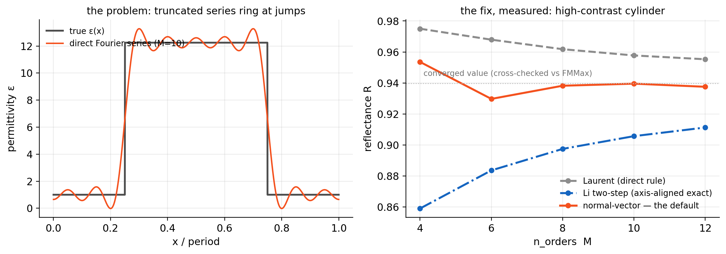
Li's inverse rule (the in-plane \(\llbracket\varepsilon\rrbracket\) in \(\mathbf{Q}\))
Writing the \(\mathbf{Q}\) above with the plain \(\llbracket\varepsilon\rrbracket\)
is Laurent's (direct) rule, and it is the wrong factorization for the
E-component that jumps across a boundary: there \(\varepsilon\) and \(E_\perp\)
both jump while \(D_\perp=\varepsilon E_\perp\) stays continuous, so the product
must be factorized with the inverse rule \(\llbracket 1/\varepsilon
\rrbracket^{-1}\) (Li, JOSA A 13, 1870 (1996)). Using the direct rule
instead leaves an \(\mathcal{O}(1/M)\) Gibbs error that cripples TM /
high-contrast convergence. Li's two-step (separable) operator (JOSA A 14,
2758 (1997)) — \(\llbracket 1/\varepsilon\rrbracket^{-1}\) along the normal axis,
direct rule along the tangential one (_mixed_convolution) — fixes this
exactly for axis-aligned boundaries (factorization="li"). The longitudinal
\(\llbracket\varepsilon\rrbracket^{-1}\) in \(\mathbf{P}\) is already
inverse-rule-correct and is unchanged.
The normal-vector method (the default, factorization="auto")
Li's two-step rule splits the inverse rule along the fixed x and y axes,
which is only correct when boundaries run along those axes. A curved or
oblique boundary has its discontinuity along the local normal, so the
separable rule mis-factorizes it — leaving a residual error that no amount of
\(n_\text{orders}\) removes (e.g. a high-index ring can sit ~2 % off the true
reflectance). The normal-vector method (Fast Fourier Factorization;
Schuster et al., JOSA A 24, 2880 (2007); Liu & Fan, JOSA A 29,
2350 (2012)) builds a smooth unit vector field that follows the true boundary
normal everywhere and applies the inverse rule along that direction, giving
the full in-plane permittivity tensor (with off-diagonal terms) in
\(\mathbf{Q}\). Ikarus constructs the tangent field by double-angle orientation
diffusion and assembles the tensor in _normalvector.py; on axis-aligned
geometry the field is constant and it collapses exactly back to "li".
This is the default, validated against FMMax's Formulation.NORMAL to
\(\le 2\times10^{-3}\) on cylinders, rings, ellipses and rotated shapes.
For anisotropic patterned layers the same idea is applied via the rotated
form of Liu & Fan eq. 45: the in-plane tensor is rotated pointwise into local
(tangent, normal) coordinates, factorized there (inverse rule on the
normal-normal entry, Laurent elsewhere), and rotated back in Fourier space. One
caveat: the tensor formulation is not strictly energy-conserving at finite
order, so energy_balance shows a small deviation that shrinks to 0 with
convergence — a more honest signal than the separable rule, which can report
perfect energy balance while still biased on a curved boundary.
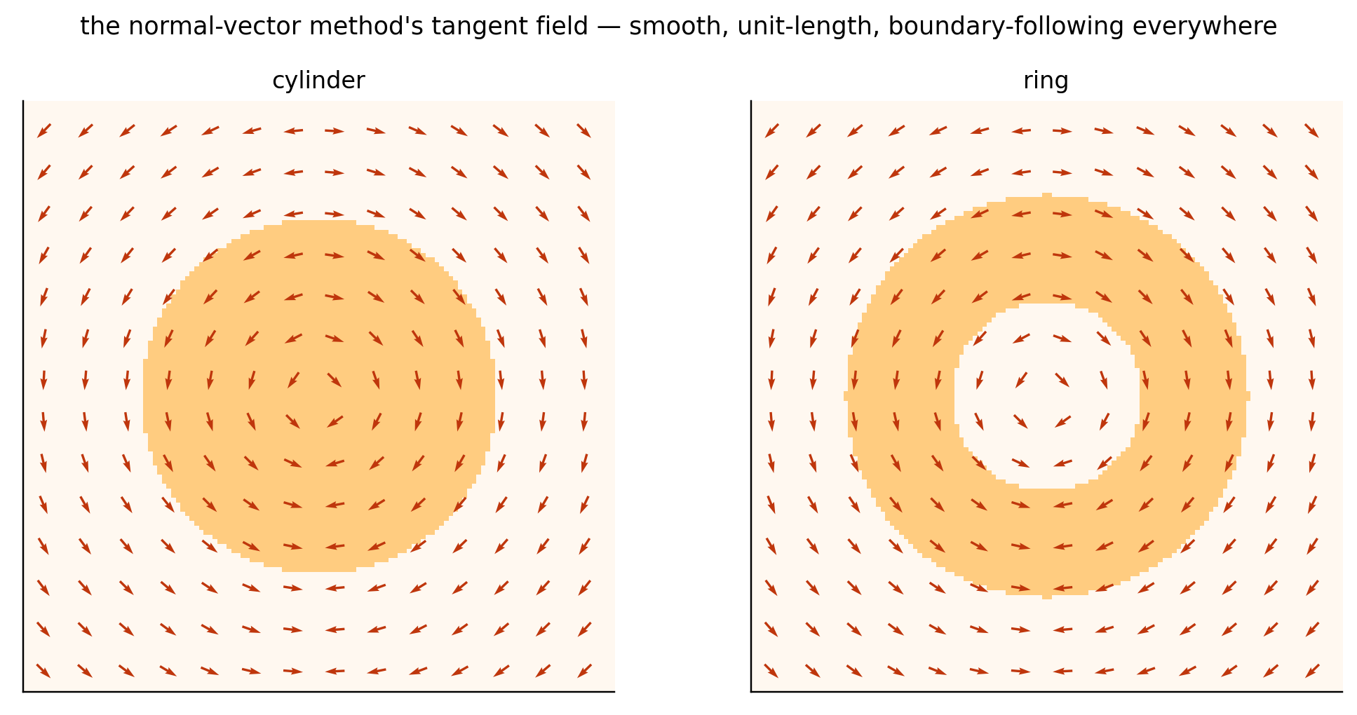
ikarus.core._normalvector.tangent_field).
The inverse rule is applied along the local normal it defines — that single
idea is what the right panel above is measuring.Scattering matrices and the star product
A scattering matrix relates incoming mode amplitudes on both sides of a block to outgoing ones:
Show me the single-layer S-matrix
Referencing each layer to a common gap medium, with
the layer blocks follow the standard Rumpf expressions. The crucial property: \(\mathbf{X}\) only ever appears with the negative exponent — every entry is bounded, no matter how thick \(L\) or how evanescent \(\lambda\).
Adjacent blocks combine with the Redheffer star product (redheffer_star):
whose \((\mathbf{I} - \mathbf{S}^B_{11}\mathbf{S}^A_{22})^{-1}\)-type factors
are exactly the resummed geometric series of inter-layer reflections — the
infinite ping-pong, settled in closed form. Ikarus evaluates these with
scipy.linalg.solve (right-division), so no explicit matrix inverse is ever
formed in the hot path. Cascading reflection region, layers and transmission
region gives the global S-matrix, and then
From amplitudes to answers
The power down exit lane \((m,n)\) is its longitudinal Poynting flux relative to the incident wave:
analogously for \(T_{mn}\). The totals obey \(R_{\text{total}} + T_{\text{total}} = 1\) for a lossless stack — Ikarus treats the defect \(|R+T-1|\) as a built-in lie detector for convergence and sign errors, and warns you automatically when the books don't balance.
Part III — The fine print
Polarization conventions
Ikarus uses the physics \(\exp(-i\omega t)\) time convention throughout its public API. The incident direction is set by polar angle \(\theta\) (from \(+z\)) and azimuth \(\phi\) (from \(+x\)); the transverse basis is
- \(\hat{\mathbf{a}}_{\text{TE}} = \hat{\mathbf{z}} \times \hat{\mathbf{k}}\) (s-polarization),
- \(\hat{\mathbf{a}}_{\text{TM}} = \hat{\mathbf{a}}_{\text{TE}} \times \hat{\mathbf{k}}\) (p-polarization).
| You ask for | You get |
|---|---|
linear, linear_pol_angle = ψ |
\(\cos\psi\,\hat{\mathbf{a}}_{\text{TE}} + \sin\psi\,\hat{\mathbf{a}}_{\text{TM}}\) — 0 = TE/s, 90 = TM/p |
RCP |
\((\hat{\mathbf{a}}_{\text{TE}} + i\,\hat{\mathbf{a}}_{\text{TM}})/\sqrt{2}\) |
LCP |
\((\hat{\mathbf{a}}_{\text{TE}} - i\,\hat{\mathbf{a}}_{\text{TM}})/\sqrt{2}\) |
At normal incidence TE/TM is degenerate, so Ikarus pins
\(\hat{\mathbf{a}}_{\text{TE}} = +\hat{\mathbf{y}}\) and
\(\hat{\mathbf{a}}_{\text{TM}} = +\hat{\mathbf{x}}\) — linear_pol_angle
becomes the literal E-field angle in the xy-plane. For circular light, the
zero order is reported as a co/cross handedness decomposition normalized so
\(|c_{\text{co}}|^2 + |c_{\text{cross}}|^2\) equals the order's efficiency.
Comparing phase against another tool?
Conventions differ between codes (time sign, reference plane). Expect a possible sign flip and/or constant offset; compare the dispersion — the shape of phase vs. wavelength — not absolute values. In our grcwa cross-check the offset was a constant \(\approx -\pi\) and the dispersion agreed to ~21 mrad.
Material models
A material is its complex permittivity \(\varepsilon(\lambda) = (n + ik)^2\). Under \(\exp(-i\omega t)\), absorbers have \(k > 0\), \(\mathrm{Im}(\varepsilon) > 0\) — feed Ikarus gain-signed data and the energy balance will politely exceed 1 to tell you. Three model types (full API: Layers & Materials):
- Tabulated \(n(\lambda), k(\lambda)\) — cubic-spline interpolated (linear below 4 points), extrapolated by clamping to the nearest endpoint.
- Lorentz oscillators: (\varepsilon(\omega) = \varepsilon_\infty
- \sum_j f_j\,\omega_{0j}^2 / (\omega_{0j}^2 - \omega^2 - i\gamma_j\omega)).
- Constant index — any bare number you pass as a material.
How many harmonics is enough?
The truncation \(M\) is the accuracy/cost dial, and the cost is steep: the eigensolve scales as \(\mathcal{O}(P^3)\). The convergence folklore, which Ikarus's own validation reproduces:
- TE and gentle structures: fast convergence, \(M \sim 8\!-\!12\) often suffices.
- TM, high contrast, metals: historically slow — the normal \(D\)-field is
discontinuous at boundaries and a directly-factorized series rings (Gibbs). The
default normal-vector factorization removes that error along the
true local boundary normal, so these now converge at \(M \sim 8\!-\!15\) instead
of \(30+\) — including on curved/oblique boundaries where the older separable
rule stays biased. Pass
factorization="laurent"to see the old slow behaviour. - Always watch \(|R+T-1|\) (lossless cases) and that \(R\)/phase have stopped
moving — energy can balance while an unconverged result still drifts. Use the
convergence tools or
simulate(auto_converge="once").
Branch selection and stability
A war story worth knowing. For a lossless evanescent order, the modal
eigenvalue argument is real and negative, and a naive square root can land
on the wrong Riemann branch — silently flipping the sign of evanescent
magnetic-mode columns. The cruelty: the bug is invisible for thin films
(only the zero order propagates) and catastrophic for every diffraction
grating. Ikarus selects the forward/decaying branch with one consistent rule
across the gap medium, the semi-infinite regions and all patterned layers
(_forward_branch, uniform_modes), and adds a vanishing imaginary loss to
regularize orders sitting exactly on a Rayleigh–Wood anomaly (the light
line). Both fixes are locked in by the validation suite.
Limitations of RCWA
Honesty corner. RCWA is exact as \(M \to \infty\) for layered periodic media, but the practical method — and this implementation — has edges:
| Limitation | What it means for you |
|---|---|
| Staircase approximation | Curved/slanted sidewalls are pixelated; approximate slopes by slicing into several thin layers. |
| Curved-boundary factorization | Handled: the default normal-vector method (Fast Fourier Factorization) applies the inverse rule along the true local boundary normal, so curved/oblique high-contrast in-plane boundaries converge correctly (validated against FMMax). It is not strictly energy-conserving at finite order — a small energy_balance deviation that vanishes with n_orders. |
| Anisotropy: in-plane + z only | Birefringent media are supported as [[eps_xx, eps_xy, 0], [eps_yx, eps_yy, 0], [0, 0, eps_zz]] — any in-plane optic axis plus a distinct z response (wave plates, c-plates, patterned birefringence). Tilted-optic-axis media (eps_xz/eps_yz) and magneto-optic gyrotropy are not supported; the cover and substrate must be isotropic. |
| Strict periodicity | Isolated objects need a padded supercell. |
| One frequency per solve | Broadband = sweep wavelengths. No time-domain output. |
| CPU only | No GPU backend; see Need for Speed for what to do instead. |
Further reading
The canonical papers behind the method are collected in Citation → Background references — Moharam & Gaylord's original formulation, Li's factorization and S-matrix recursion analyses, and Rumpf's convention-consistent scattering-matrix formulation, which Ikarus follows.
Machinery understood. Now go bend some light: Flight School →