Need for Speed¶

What a solve costs, where the time goes, and the two tricks worth an order of magnitude.

The price of harmonics¶

Everything is governed by one number — the harmonic count

\[ P = (2M_x + 1)(2M_y + 1) \]

for n_orders = (Mx, My). Each patterned layer demands one dense eigendecomposition of a \(2P \times 2P\) matrix, and the scattering algebra moves \(2P \times 2P\) blocks around. So, per layer:

\[ \text{time} \sim \mathcal{O}(P^3), \qquad \text{memory} \sim \mathcal{O}(P^2). \]

Read that cubic again: doubling \(M\) in 2-D quadruples \(P\) and costs you ~64× the time. The consequences, in order of importance:

n_orders is the throttle. Find the smallest converged value (the ritual) and stop.
1-D gratings fly economy for free: n_orders=(M, 0) gives \(P = 2M+1\) — linear, not quadratic.
Uniform layers cost nothing. Their modes are analytic; a thin-film stack at n_orders=0 is effectively instant.

Indicative single-solve timings¶

One 2-D solve of a patterned layer, single thread — orders of magnitude, not a contract (your CPU and BLAS will vary):

\(M\)	harmonics \(P\)	matrix size \(2P\)	time
5	121	242	~0.1 s
8	289	578	~0.4 s
9	361	722	~1 s
12	625	1250	~4 s
13	729	1458	~8 s
15	961	1922	~20 s

From \(M=9\) to \(M=13\): \(P\) doubles, time ×8. The cube never sleeps.

How Ikarus stacks up

Head-to-head against the independent grcwa (both tools fed byte-identical material data), Ikarus agreed on \(R\), \(T\) and phase to ~10⁻³ while running ~1.5–1.7× faster per solve (729 harmonics: ~8 s vs ~13 s). The margin comes from exploiting identity gap modes (\(W_0 = I\)), diagonal algebra in homogeneous regions, and scipy.linalg.solve right-division instead of explicit inverses.

Convergence of the energy defect — Energy-conservation defect |R+T−1| vs. harmonic count for a high-contrast aSi square in TM — the slow-converging regime.

Memory scaling¶

The heavyweights are \(2P \times 2P\) complex128 matrices — several live per patterned layer at \((2P)^2 \times 16\) bytes apiece:

\(M\)	\(2P\)	one matrix
5	242	~0.9 MB
8	578	~5 MB
10	882	~12 MB
12	1250	~25 MB
15	1922	~59 MB
20	3362	~181 MB

Budget a handful per layer. Deep stacks at large \(M\): lower n_orders, or run fewer solves simultaneously.

BLAS threading¶

The most impactful knob in the whole chapter — and it's two lines.

Tight loops of small solves (sweeps, GA populations): the matrices are too small for threaded BLAS to win; it burns the time spawning and synchronizing threads instead. Pin one thread per process and parallelize at the process level:

import os
for v in ("OMP_NUM_THREADS", "OPENBLAS_NUM_THREADS",
          "MKL_NUM_THREADS", "VECLIB_MAXIMUM_THREADS"):
    os.environ.setdefault(v, "1")
import numpy as np  # noqa: E402 — must come AFTER the env vars

In our testing this made an inverse-design run roughly an order of magnitude faster on a many-core machine. Not a typo.

Large single solves (\(M \gtrsim 20\)): the opposite regime — one eigendecomposition is big enough to feed every core. Let BLAS thread, parallelize coarser. When in doubt, benchmark both; it takes two minutes.

Convergence cheat sheet¶

Structure	Typical `n_orders`	Notes
Thin films (uniform)	`0`	exact, instant
Gentle dielectric metasurfaces	8–12	TE and TM both quick
High-contrast dielectric	12–18	verify TM specifically
Metals, TM / p-pol	18–30+	the slow lane — see below
1-D gratings	`(15–30, 0)`	cheap because 1-D

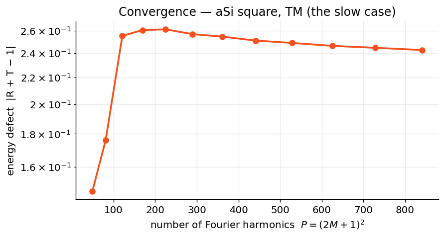
Always converge at your worst-case wavelength/polarization, watching \(|R+T-1|\) for lossless structures.

The Laurent tax

Ikarus factors the permittivity with Laurent's rule. The accelerated Li inverse rule — which tames TM convergence at sharp high-contrast/metallic edges — is not yet implemented, so those problems need more harmonics here than in a Li-rule code. Known roadmap item (Theory → Limitations).

Accuracy ledger¶

Analytic Fresnel/transfer-matrix agreement: ~10⁻¹⁵, any angle, any polarization.
Energy conservation, lossless gratings: ~10⁻⁹.
Under-sampled geometry fails loudly (a ValueError from the convolution matrix), never silently — resolution is auto-raised to ≥ 4M+1.
Near Rayleigh–Wood anomalies: tiny regularization loss, locally elevated energy defect, slower convergence. Refine n_orders if your metric lives there.

The pre-takeoff checklist¶

[x] Smallest converged n_orders (run the ritual, then stop turning the dial)
[x] 1-D problems declared 1-D; thin films at n_orders=0
[x] BLAS pinned to 1 thread for sweeps/optimization; processes for parallelism
[x] One RCWA reused across a sweep — only the source changes
[x] energy_balance glanced at after every structural change