Lesson 3 · Sculpting Wavefronts

Mission: build a 2-D meta-atom from shape primitives, harvest the transmission phase (the metasurface designer's currency), and look at the near field with your own eyes.

A dielectric nanopillar

A square lattice of TiO₂ cylinders on glass — the canonical building block of visible-light metalenses:

import numpy as np
from ikarus import RCWA, shapes

period = 420e-9
N = 128
pillar = shapes.circle(center=(0.5, 0.5), radius=0.32, grid_shape=(N, N))

rcwa = RCWA(period_x=period, period_y=period, resolution=(N, N), n_orders=(10, 10))
rcwa.add_uniform_layer(np.inf, "Air")
rcwa.add_layer(600e-9, pillar, ["Air", "TiO2"])   # 0 -> Air, 1 -> TiO2
rcwa.add_uniform_layer(np.inf, "SiO2")
rcwa.set_source(wavelength=532e-9, theta=0, polarization="linear")

_, _, res = rcwa.simulate()
print(f"T={res.T_total:.3f}  R={res.R_total:.3f}  R+T={res.energy_balance:.5f}")

See what you built:

rcwa.visualize_structure(plane="xz", savefig="stack.png")          # the stack
rcwa.visualize_structure(plane="xy", layer_index=1, savefig="topology.png")

Phase: the designer's currency

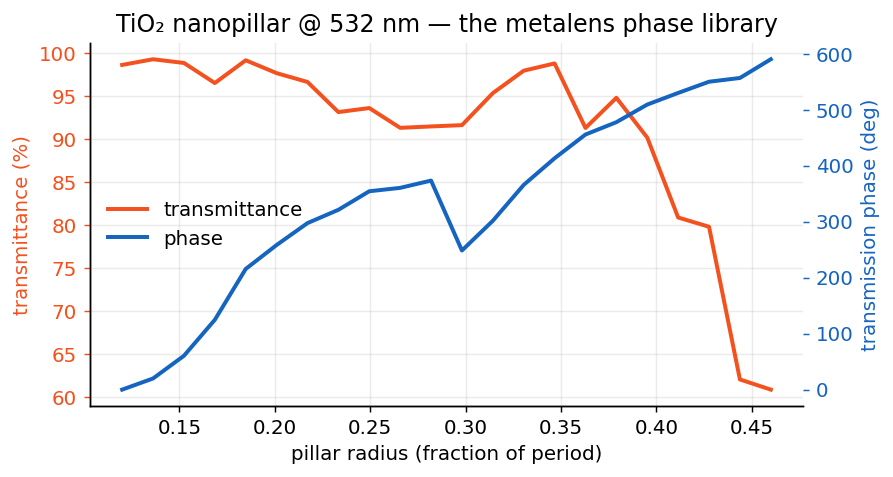
A metalens is a map from position to phase delay. You build it from a library of pillars whose radius tunes the transmission phase of the specular order — ideally covering a full \(2\pi\) while staying transparent:

radii = np.linspace(0.15, 0.45, 25)
T, phase = [], []
for r in radii:
    pillar = shapes.circle(radius=r, grid_shape=(N, N))
    rcwa = RCWA(period_x=period, period_y=period, resolution=(N, N), n_orders=(10, 10))
    rcwa.add_uniform_layer(np.inf, "Air")
    rcwa.add_layer(600e-9, pillar, ["Air", "TiO2"])
    rcwa.add_uniform_layer(np.inf, "SiO2")
    rcwa.set_source(wavelength=532e-9, theta=0, polarization="linear")
    _, _, res = rcwa.simulate()
    T.append(res.T_total)
    phase.append(res.T_phase)             # zero-order phase, radians

phase = np.unwrap(phase)
print(f"phase coverage: {np.degrees(phase.ptp()):.0f} deg "
      f"(a full library wants >= 360)")

Each pillar is a tiny truncated waveguide; fatter pillar → higher effective index → more phase delay. When the sweep covers \(2\pi\) with \(T \gtrsim 0.9\), you have a complete set of "phase pixels" to tile any wavefront you like.

Sweeping the pillar radius scans the transmission phase across a full 2π while transmittance stays high — the meta-atom phase library.

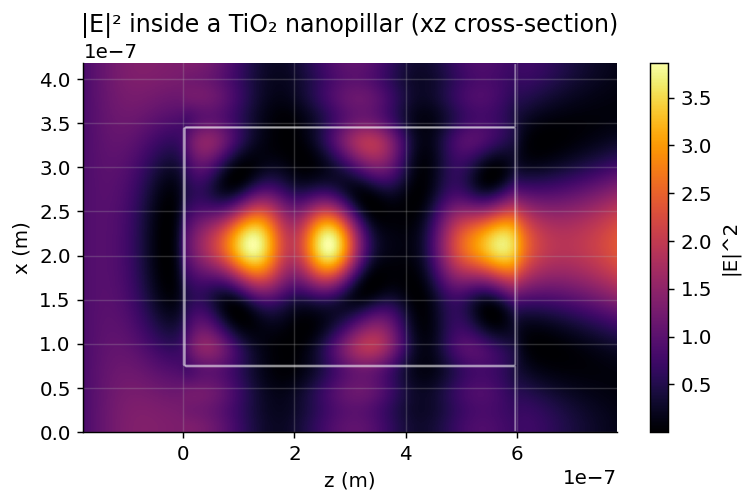
Near-field maps

Numbers are good; seeing the Mie resonance inside the pillar is better:

from ikarus.visualization import plot_field

rcwa.set_source(wavelength=532e-9)
rcwa.simulate()

# xz cross-section through the pillar center:
xz = rcwa.get_fields(plane="xz", nx=160, y_position=period / 2)["xz"]
ax = plot_field(xz, component="intensity")          # |E|² + structure outline
ax.figure.savefig("pillar_field_xz.png", dpi=150, bbox_inches="tight")

# xy slice at mid-height:
xy = rcwa.get_fields(z_positions=[300e-9], plane="xy", nx=160, ny=160)
ax = plot_field(list(xy.values())[0], component="intensity")
ax.figure.savefig("pillar_field_xy.png", dpi=150, bbox_inches="tight")

The plots come with the material outline overlaid automatically, so you can check the field actually lives where you think it does.

Reconstructed |E|² through the TiO₂ nanopillar (xz cross-section), with the material outline overlaid automatically.

Too lazy to sweep radii? Good.

Declaring the goal and letting a genetic algorithm sculpt the meta-atom is a one-liner away — see Inverse Design and the broadband AR coating in The Hangar.

Expected results

• High transmittance (T ≳ 0.9) away from resonances, with dips at the pillar's Mie resonances.
• A phase ramp vs. radius spanning ≥ 360° for a well-chosen height — your metalens alphabet.

Pilot habits

• Keep the period subwavelength in the substrate (period < λ/n_sub) so no stray diffraction lanes open — all the power stays in the specular order you're phase-engineering.
• n_orders 8–12 is the dielectric-pillar sweet spot; confirm with Lesson 4's convergence ritual.
• Reconstruct fields on a finer nx/ny than the solver resolution — the reconstruction grid is free to choose.

---

Next: Lesson 4 · Sweeping Gracefully →