Lesson 7 · Inverse Design

Mission: stop choosing parameters by hand. State a goal — "maximum transmission at 1300 nm", "reflect 1064 and 1550", "show me the trade-off" — and let the optimizer design the meta-atom for you: named shape parameters, fully freeform pixel patterns, heights, periods, or several of these at once.

Every previous lesson was forward design: you set the geometry, Ikarus told you the optics. This one runs the arrow backwards — five ways.

Two ways to hold a degree of freedom

Ikarus's inverse module (ikarus.inverse) optimizes two kinds of topology DOF — and optimize() automatically picks the right engine for each (you never choose):

DOF	What it is	Engine optimize() picks
Parametric shape	a shape class (Cross, SplitRing, …) with named, bounded parameters	genetic algorithm — a few interpretable knobs, and rasterization has no gradients
Pixel map	a free binary grid (pixels(nx, ny, symmetry=...))	adjoint gradients — the derivative w.r.t. every pixel costs about one extra solve, so freeform scales to thousands of DOFs

The first half of this lesson is the parametric route — the one your intuition can read. The second half goes freeform.

Extras

Parametric/GA route: pip install "ikarus-rcwa[inverse]" (pymoo). Freeform/adjoint route: pip install "ikarus-rcwa[grad]" (JAX). [all] includes both.

Parametric shapes

A parametric Shape carries named parameters and a rotation angle. Used normally, it's just a tidy topology:

from ikarus.shapes import Cross
topo = Cross(arm_length=0.7, arm_width=0.2, angle=30).to_grid((128, 128))

The trick: any parameter may be a free(lo, hi) range instead of a number. Mark a few free, and they become the optimization variables — no pixel grids, no loss of physical meaning.

from ikarus.inverse import free
from ikarus.shapes import Cross

shape = Cross(arm_length=free(0.3, 0.95),   # free: the GA will choose
              arm_width=free(0.1, 0.45),    # free
              angle=free(0, 90))            # free: rotation is a knob too
shape.free_parameters()
# {'angle': (0.0, 90.0), 'arm_length': (0.3, 0.95), 'arm_width': (0.1, 0.45)}

The three-step recipe

Declare the meta-atom, state the target, optimize:

import os
os.environ.setdefault("OMP_NUM_THREADS", "1")   # single-thread BLAS for the GA loop

from ikarus.inverse import MetaAtom, free, optimize, Target
from ikarus.shapes import Cross

# 1. a Si cross on glass whose arms, rotation and height are all free
atom = MetaAtom(period=700e-9, cover="Air", substrate="SiO2")
atom.add_pattern(topology=Cross(arm_length=free(0.3, 0.95),
                                arm_width=free(0.1, 0.45),
                                angle=free(0, 90), grid_shape=(96, 96)),
                 materials=["Air", "Si"],
                 height=free(0.3e-6, 0.9e-6))

# 2. what we want: maximum transmission at 1300 nm
target = Target.maximize("T", at=1300e-9)

# 3. evolve it
best = optimize(atom, target, n_orders=6, pop=16, n_gen=10, seed=0)
print(best.report())            # achieved T, in metric units
best.plot()                     # convergence curve, one line

design = best.metaatom          # a ready-to-simulate RCWA

The optimizer enumerates the free shape parameters automatically — they appear in the report as shape__arm_length, shape__angle, and so on, alongside the free height:

Inverse-design result:
  max(T):  T = 1.0002   (loss = -0.00021)  [ga]
    height = 7.64e-07
    shape__angle = 69.66
    shape__arm_length = 0.4247
    shape__arm_width = 0.1382

The genetic algorithm chose the arm dimensions, rotation and height of a Si cross to maximize transmission at 1300 nm (dotted line). Left: the evolved topology. Right: its full spectrum, computed by Ikarus.

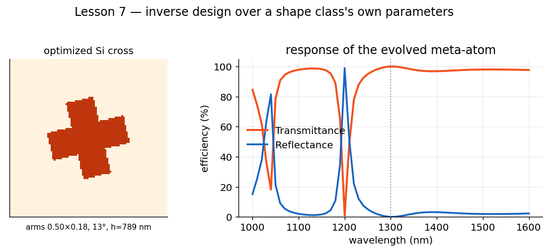
Plot the result

Visualize the evolved meta-atom and sweep its spectrum:

import numpy as np
import matplotlib.pyplot as plt

design = best.metaatom            # the optimized RCWA (also best.rcwa)

# the evolved topology (the patterned layer is layer 1)
design.visualize_structure(plane="xy", layer_index=1, savefig="evolved_atom.png")

# its transmission spectrum
wl = np.linspace(1.0e-6, 1.6e-6, 31)
T = []
for w in wl:
    design.set_source(wavelength=w, theta=0, polarization="linear")
    T.append(design.simulate()[2].T_total)

plt.figure(figsize=(7, 4))
plt.plot(wl * 1e9, np.array(T) * 100, lw=2)
plt.axvline(1300, color="0.6", ls=":")        # the optimization target
plt.xlabel("wavelength (nm)"); plt.ylabel("transmittance (%)")
plt.title("Spectrum of the evolved meta-atom"); plt.grid(alpha=0.3)
plt.tight_layout(); plt.savefig("evolved_spectrum.png", dpi=150, bbox_inches="tight")
plt.show()

Going freeform: pixels + adjoint gradients

When you have no good shape prior, hand the optimizer a blank pixel canvas. The call is the same — only the topology changes. A beam deflector (steer the reflected power into the +1 order — a job that requires structure; runs in a few minutes):

from ikarus.inverse import MetaAtom, optimize, pixels, Target

atom = MetaAtom(period=2000e-9, cover="Air", substrate="SiO2")
atom.add_pattern(topology=pixels(64, 64, symmetry="mirror_y"),  # 2,048 DOFs
                 materials=["Air", "aSi"], height=500e-9)

best = optimize(atom, Target.maximize("R", at=1550e-9, order=(1, 0)),
                n_orders=8, min_feature=100e-9,   # fab-ready feature-size limit
                init="random", restarts=4,        # steering is multi-modal: multistart
                verify_n_orders=16)               # report at a converged truncation
print(best.report())                              # achieved R(+1,0), honest units
best.plot()                                       # convergence curve, one line
best.rcwa.visualize_structure(plane="xy", layer_index=1)  # the invented topology

Because the problem is differentiable, optimize() silently switches from the GA to adjoint gradients: each iteration computes the derivative of the objective with respect to every pixel at once for the price of roughly one extra solve. Pixels are optimized as continuous densities, smoothed by a minimum-feature filter (min_feature, in meters — your fab's design rule), sharpened toward binary as the run progresses, and the final hard-binarized design is re-verified with the standard solver at the optimization n_orders, so best.F matches best.rcwa.simulate() there. That number is honest but not necessarily converged: optimize() re-checks at a higher truncation and warns if the metric is still moving -- pass verify_n_orders= to report at a converged order (energy balance ~1 will not flag this; only an n_orders sweep does).

When does each engine actually win?

We measured it, honestly — same problems, hard-binarized designs re-verified at a higher truncation than either optimizer used:

The crossover is the lesson. Left: a toy 1-D deflector (40 pixels) — both engines finish in seconds, and the genetic algorithm legitimately wins: a few hundred evaluations can genuinely search a space that small. (The adjoint curve's late start is one-time JAX compilation — at freeform scale it amortizes to nothing.) Right: the same physics at freeform scale (2,048 pixels; the adjoint got ten minutes, the GA got twice that) — the adjoint's whole-gradient steps dominate, because the gradient's cost doesn't grow with the pixel count but the GA's search space explodes. 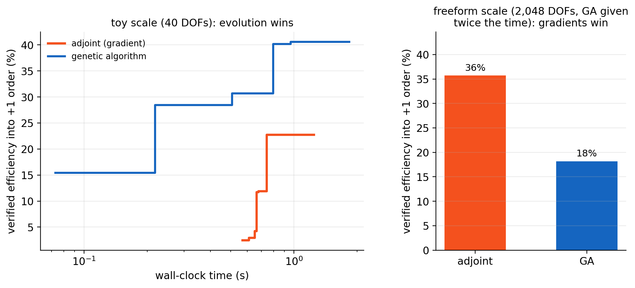Small discrete spaces belong to evolution; freeform scale belongs to gradients — which is exactly why optimize() keeps both engines.

The continuous knobs: heights and periods

Not every design question is a topology question. Layer height and the period can be free(...) too — and because they are smooth, differentiable quantities, optimize() again uses adjoint gradients. A case with a textbook answer, so you can watch the optimizer be exactly right (runs in seconds):

import numpy as np
from ikarus.inverse import MetaAtom, Target, optimize, free

# a quarter-wave AR candidate: index sqrt(1.5) film on glass, height free
atom = MetaAtom(period=400e-9, cover="Air", substrate=1.5)
atom.add_pattern(topology=np.zeros((4, 4), dtype=int), materials=[1.2247],
                 height=free(60e-9, 200e-9))

best = optimize(atom, Target.minimize("R", at=600e-9), n_orders=1)
print(best.report())
# height -> 122.5 nm  ==  lambda / 4n, the analytic optimum, and R ~ 1e-9

One design, several wavelengths: worst-case targets

"High reflectance at 1064 nm and 1550 nm, from the same atom" is one objective — the worst of the two wavelengths — not two separate ones. Say exactly that with worst_case=True, and it stays on the adjoint fast path (pixels and the free height are optimized together):

from ikarus.inverse import MetaAtom, Target, optimize, free, pixels

atom = MetaAtom(period=900e-9, cover="Air", substrate="SiO2")
atom.add_pattern(topology=pixels(40, 40, symmetry="c4v"),
                 materials=["Air", "aSi"], height=free(300e-9, 800e-9))

target = Target.maximize("R", at=[1064e-9, 1550e-9], order=None,
                         worst_case=True)          # lift the WORST wavelength
best = optimize(atom, target, n_orders=8, min_feature=80e-9,
                init="random", restarts=3)         # symmetric start is a trap
print(best.report())
# -> worst-case R ≈ 0.92 (R@1064 ≈ 0.92, R@1550 ≈ 0.98); ~10 min for 3 restarts

A uniform-gray start is a trap here — use init="random"

From the default 50 %-everywhere density this symmetric objective has zero gradient and the optimizer never moves (worst-case R frozen near 3 %). The init="random" + restarts=3 above breaks the symmetry and lands at ~92 %. This is the same multi-modal-landscape lesson as the deflector: whenever a run's loss is flat from step 0, restart from noise.

Under the hood the adjoint engine uses a smoothed maximum so both wavelengths receive gradient every step (a hard max would starve the currently-better one) — but the reported objective is the honest hard worst case, re-evaluated with the standard solver.

Trade-offs on purpose: Pareto fronts (NSGA-III)

Sometimes you don't want one compromise — you want to see the whole trade-off. Pass two or more Targets and optimize() switches to NSGA-III, which returns the Pareto front in a single run (this is the one thing gradients cannot do: one adjoint run yields one point on that front, not the curve):

atom = MetaAtom(period=900e-9, cover="Air", substrate="SiO2")
atom.add_pattern(topology=pixels(24, 24, symmetry="c4v"),
                 materials=["Air", "aSi"], height=free(300e-9, 800e-9))

targets = [Target.maximize("R", at=1064e-9, order=None),
           Target.maximize("R", at=1550e-9, order=None)]
front = optimize(atom, targets, n_orders=6, pop=60, n_gen=40)   # minutes

import numpy as np
F = np.asarray(front.F)                     # one row per Pareto design
for i, f in enumerate(F[:5]):
    print(f"design {i}:  R(1064) = {1-f[0]:.3f}   R(1550) = {1-f[1]:.3f}")

pick = front.X[2]                           # choose your compromise...
rcwa = front.atom.build(pick, n_orders=6)   # ...and simulate it

Rule of thumb: worst_case=True when you know the balance you want (and want adjoint speed); separate targets when the balance itself is the question.

Taking the controls yourself

algorithm="auto" is the default and the recommendation — but nothing is hidden. Force an engine and tune it explicitly:

best = optimize(atom, target, algorithm="adjoint",     # force gradients
                steps=300, learning_rate=0.02,         # longer, gentler
                min_feature=100e-9,                    # your fab's design rule
                beta=(8, 512))                         # binarization ramp

best = optimize(atom, target, algorithm="ga",          # force the GA
                pop=120, n_gen=100)                    # its knobs, as always

Knob	Engine	Meaning
steps, learning_rate	adjoint	Adam iterations (~1.5 solves each per wavelength) and step size.
min_feature (meters)	adjoint	conic-filter radius = half this; keeps pixel designs fabbable and smooths the landscape.
beta=(lo, hi)	adjoint	sharpness ramp pushing densities to binary.
restarts	adjoint	run N random-seeded restarts, keep the best (steering objectives are multi-modal -- not optional there).
verify_n_orders	both	report/verify the final design at a higher truncation; a convergence warning fires by default.
init	adjoint	pixel start: "uniform" (default — reflect/transmit objectives), "random" (deflection/steering objectives, whose landscape is flat at uniform gray — run a few seeds and keep the best), or a float fill.
pop, n_gen	GA family	population and generations.
seed	both	reproducible runs.

If you pass GA knobs to a problem that auto-routes to adjoint, Ikarus warns and ignores them — pass algorithm="ga" if you really meant the GA.

The engine map

Your problem	Engine auto picks	Why
Freeform pixels(...), one target	adjoint	whole-gradient per solve; scales to thousands of DOFs
Free height / period, one target	adjoint	smooth, differentiable
One target over several wavelengths (worst_case or mean)	adjoint	still a single scalar objective
Parametric Shape DOFs	GA	rasterization has no gradients
≥ 2 targets (the trade-off is the question)	NSGA-III	a full Pareto front in one run
Structure stacks, anisotropic materials, circular-pol coefficient targets	GA	not yet on the differentiable path
[grad] extra not installed	GA	graceful fallback

Many real workflows chain the engines: parametric GA to get close and understand the physics, freeform adjoint to squeeze the last percent.

Bringing your own shape class

add_layer and the inverse module accept any object that exposes an img array (or a to_grid() method), so an external topology library drops straight in:

# any class with a binary `.img` numpy array works as a topology
rcwa.add_layer(200e-9, MyTopologySpecies(lx=0.4, ly=0.7), ["Air", "Si"])

To make a custom shape optimizable, subclass ikarus.shapes.Shape: declare its parameters in _PARAMS and implement _mask. It then inherits free_parameters, rotation and the inverse-design plumbing for free.

Expected results

• A converging objective (the GA's f_min drops each generation), ending in a high-transmission cross with a specific rotation.
• A spectrum with the target wavelength sitting in a transmission window — and, often, a sharp resonance nearby that the optimizer steered away from the target.

Pilot habits

• Pin BLAS to one thread (why) — GA loops are many small solves.
• Start with small pop/n_gen (GA) or small steps (adjoint) to gauge runtime and sanity, then scale up.
• For pixel maps, set min_feature to your fab's design rule from the start — it also smooths the optimization landscape.
• Keep the forward model faithful to your features. Optimizers exploit whatever you give them — on an under-resolved model (n_orders too low for the pixel size) any engine will happily "optimize" numerical artifacts that vanish on a converged re-check. Chunky pixels or a min_feature matched to n_orders keep the fitness honest; always re-simulate the final design at higher n_orders before believing it.
• Beware trivial attractors. "Maximize total R" can be satisfied by a boring uniform slab — gradients will happily roll into it. Objectives that require structure (specific orders, phase targets, multi-wavelength) make far better use of the optimizer.
• For steering/deflection objectives, use init="random" (+ a few seeds): their landscape is flat at uniform gray.
• A handful of pixels? The GA is genuinely competitive (it can nearly enumerate small spaces) — the adjoint's edge grows with DOF count. Forcing algorithm="ga" on a 30-pixel problem is a perfectly good choice.
• Bound parameters physically (an arm_width can't exceed the period) — tight, honest ranges make the search both faster and manufacturable.
• Free the rotation: angle is a cheap extra knob that unlocks polarization-dependent and chiral responses (try SplitRing).

---

Next: Lesson 8 · Stacking the Deck → — optimize a whole multi-layer stack at once.