Lesson 4 · Sweeping Gracefully

Mission: sweep parameters without wasting a single eigensolve (or writing a single for-loop you don't have to), perform the convergence ritual every trustworthy result rests on, and paint a 2-D design map.

The easy way: Sweep

For source sweeps — wavelength, angle, polarization — skip the loop entirely. Sweep varies the source over a grid and hands back arrays, with one progress bar for the whole run (so you can see the ETA):

import numpy as np
from ikarus import RCWA, shapes, Sweep

period, N = 450e-9, 96
disk = shapes.circle(radius=0.3, grid_shape=(N, N))
rcwa = RCWA(period_x=period, period_y=period, resolution=(N, N), n_orders=(9, 9))
rcwa.add_uniform_layer(np.inf, "Air")
rcwa.add_layer(200e-9, disk, ["Air", "Si3N4"])
rcwa.add_uniform_layer(np.inf, "SiO2")
rcwa.set_source(wavelength=600e-9, theta=0, polarization="linear")

res = Sweep(rcwa).over(wavelength=np.linspace(400e-9, 800e-9, 81)).run()
R = res.R_total                       # array aligned to the sweep axis

A 2-D grid is the same call with two axes — and still one bar:

res = Sweep(rcwa).over(theta=np.linspace(0, 60, 31),
                       wavelength=np.linspace(400e-9, 800e-9, 81)).run()
res.R_total.shape                     # (31, 81)
res.order(1, 0, which="R")            # +1 reflected order across the grid

The manual pattern (and your toggle)

When you need full control — or you're sweeping geometry (which rebuilds the structure) — write the loop, and wrap it in progress for one bar with an on/off switch:

from ikarus import progress

wavelengths = np.linspace(400e-9, 800e-9, 81)
R = np.empty_like(wavelengths)
for i, wl in enumerate(progress(wavelengths, desc="λ", enable=True)):
    rcwa.set_source(wavelength=wl)    # set_source remembers theta & polarization
    R[i] = rcwa.simulate()[2].R_total

Changing the source is cheap. Changing the geometry triggers a fresh eigensolve — unavoidable, that's the physics changing.

The convergence ritual

Before you trust a sweep — let alone publish it — confirm the harmonic count is sufficient. The honest way is to watch a metric stop moving:

from ikarus.tools.convergence import convergence_curve

rcwa.set_source(wavelength=600e-9)
orders, defect = convergence_curve(rcwa, range(4, 21, 2), metric="energy")
harmonics = (2 * orders + 1) ** 2
for h, d in zip(harmonics, defect):
    print(f"{h:5d} harmonics: |R+T-1| = {d:.2e}")

(convergence_curve politely restores your original n_orders afterward.) Or delegate the whole ritual:

rcwa.simulate(auto_converge="once", verbose=True)   # finds & caches n_orders
print("using n_orders =", rcwa.n_orders)

Converge at your worst point, not your favorite one

TM polarization, the highest contrast, the shortest wavelength, the steepest resonance — that's where convergence is slowest. A study run at a benign wavelength is a false sense of security with extra steps.

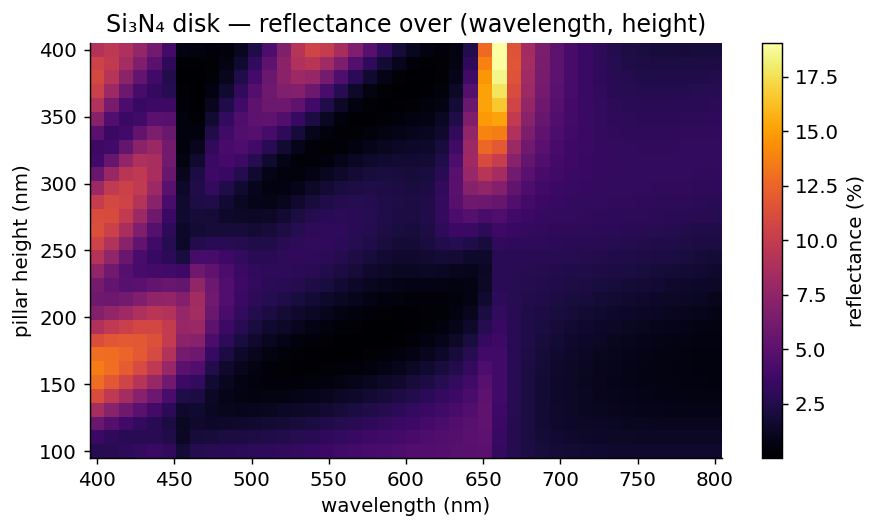
A 2-D design map

Reflectance vs. wavelength and pillar height — the kind of plot that finds designs for you. Height is structural (it rebuilds the layer), so it's the outer loop with a progress bar; wavelength is a source axis, so the inner sweep is a Sweep:

import numpy as np
from ikarus import RCWA, shapes, Sweep, progress

period, N = 450e-9, 96
disk = shapes.circle(radius=0.3, grid_shape=(N, N))
wavelengths = np.linspace(400e-9, 800e-9, 60)
heights = np.linspace(100e-9, 400e-9, 40)

Rmap = np.empty((heights.size, wavelengths.size))
for j, h in enumerate(progress(heights, desc="height")):
    rcwa = RCWA(period_x=period, period_y=period, resolution=(N, N), n_orders=(9, 9))
    rcwa.add_uniform_layer(np.inf, "Air")
    rcwa.add_layer(h, disk, ["Air", "Si3N4"])
    rcwa.add_uniform_layer(np.inf, "SiO2")
    rcwa.set_source(wavelength=600e-9, theta=0, polarization="linear")
    Rmap[j] = Sweep(rcwa).over(wavelength=wavelengths).run(progress=False).R_total

import matplotlib.pyplot as plt
plt.pcolormesh(wavelengths * 1e9, heights * 1e9, Rmap, shading="auto", cmap="inferno")
plt.xlabel("wavelength (nm)"); plt.ylabel("pillar height (nm)")
plt.colorbar(label="Reflectance"); plt.savefig("Rmap.png", dpi=150)

Resonance bands glow; anti-reflection valleys go dark. Design by sightseeing.

Reflectance of a Si₃N₄ disk over wavelength and pillar height — a 2-D design map built from nested sweeps.

Need it faster?

• Pin BLAS to one thread before importing NumPy — for these small matrices, threaded BLAS is a traffic jam, not a speedup (the full story).
• Fan out across processes — every solve is independent; Aerobatics → Batch simulations has the recipe.

Expected results

• The energy defect shrinks monotonically with n_orders; once below your tolerance (say 10⁻⁴), extra harmonics buy nothing but heat.
• The 2-D map shows resonance bands (bright R) and broadband AR valleys (dark) — the design space at a glance.

---

Next: Lesson 5 · Twisting Light →