Lesson 2 · Splitting Light

Mission: simulate a 1-D binary grating, enumerate the exit lanes light takes, and verify their angles against the grating equation — a satisfying moment of "the simulation agrees with the chalkboard."

A 1-D binary grating

A 1-D grating doesn't vary along \(y\), so we tell Ikarus both things: an (Nx, 2) topology (two identical rows) and n_orders=(M, 0) (expand x-orders only). One-dimensional physics at a one-dimensional price.

import numpy as np
from ikarus import RCWA

period = 900e-9
rcwa = RCWA(period_x=period, period_y=period, resolution=(256, 2), n_orders=(20, 0))

topo = np.zeros((128, 2), dtype=int)
topo[64:, :] = 1                      # 50% duty cycle
rcwa.add_uniform_layer(np.inf, "Air")
rcwa.add_layer(300e-9, topo, ["TiO2", "Air"])   # 0 -> TiO2, 1 -> Air
rcwa.add_uniform_layer(np.inf, "SiO2")

rcwa.set_source(wavelength=550e-9, theta=0, polarization="linear", linear_pol_angle=0.0)
_, _, res = rcwa.simulate()
print(f"R={res.R_total:.4f}  T={res.T_total:.4f}  R+T={res.energy_balance:.6f}")

TE is the easy runway

With grooves along \(y\), linear_pol_angle=0 (TE — E-field along the grooves) converges fast. 90 (TM — E-field across the grooves) is the classic slow case — but Ikarus's default Li factorization tames it, so TM converges at modest n_orders here rather than crawling (details). Still verify it has settled.

Reading the exit lanes

p, q = res.orders
print("Transmitted orders (efficiency @ exit angle):")
for i in np.argsort(-res.T_orders):
    if res.T_orders[i] > 1e-4:
        print(f"  ({p[i]:+d},{q[i]:+d}): T={res.T_orders[i]:.4f} "
              f"@ theta={res.theta_out_trn[i]:5.1f} deg")

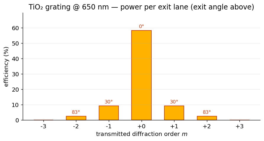
# plot the power in each transmitted order as a bar chart
import matplotlib.pyplot as plt
orders = range(-3, 4)
effs = [res.T_orders[res.order_index(m, 0)] * 100 for m in orders]
plt.figure(figsize=(7, 4))
plt.bar([f"{m:+d}" for m in orders], effs, color="C1", edgecolor="k")
plt.xlabel("transmitted diffraction order $m$"); plt.ylabel("efficiency (%)")
plt.title("Power per exit lane"); plt.grid(axis="y", alpha=0.3)
plt.tight_layout(); plt.savefig("grating_orders.png", dpi=150, bbox_inches="tight")
plt.show()

Propagating lanes get real angles; evanescent ghosts get NaN.

Power per transmitted diffraction order for the TiO₂ grating at 550 nm; the label above each bar is that lane's exit angle.

Checking against the chalkboard

At normal incidence, transmitted order \(m\) exits the substrate (index \(n_t\)) at

\[ \sin\theta_{t,m} = \frac{m\,\lambda}{n_t\,\Lambda}. \]

from ikarus import default_library
n_t = default_library.get("SiO2", 550e-9).real

for m in (-1, 0, 1):
    i = res.order_index(m, 0)
    if np.isfinite(res.theta_out_trn[i]):
        predicted = np.degrees(np.arcsin(m * 550e-9 / (n_t * period)))
        # theta_out_* is an unsigned polar magnitude (the +/- direction
        # lives in phi_out_*), so compare against |predicted|.
        print(f"order {m:+d}: Ikarus {res.theta_out_trn[i]:6.2f} deg, "
              f"grating eq {abs(predicted):6.2f} deg")

They agree to numerical precision. (The angles come from geometry alone; the efficiencies are where RCWA earns its keep.)

Watching lanes open and close

As \(\lambda\) crosses \(\Lambda/n\), higher orders switch on and off — Rayleigh–Wood anomalies, the traffic reports of grating physics:

for wl in (450e-9, 550e-9, 650e-9, 750e-9):
    rcwa.set_source(wavelength=wl)
    _, _, res = rcwa.simulate()
    n_prop = int(np.sum(np.isfinite(res.theta_out_trn) & (res.T_orders > 1e-6)))
    print(f"lambda={wl*1e9:.0f} nm: {n_prop} propagating transmitted orders, "
          f"R+T={res.energy_balance:.6f}")

Expected results

• R+T ≈ 1 to ~10⁻⁶ or better (this stack is lossless).
• Exit angles match the grating equation exactly.
• The order count changes with wavelength; near an anomaly, convergence slows a touch — normal.

Pilot habits

• Keep 1-D problems 1-D: (Nx, 2) topology + n_orders=(M, 0). A full 2-D expansion of a 1-D grating is the most common self-inflicted slowdown.
• Run your convergence study in TM — it's the demanding passenger.
• The shipped version of this lesson: python -m ikarus.examples.grating_diffraction.

---

Next: Lesson 3 · Sculpting Wavefronts →